// Twitter Cards // Prexisting Head The Biologist Is In: December 2015

Tuesday, December 29, 2015

Biological Patterns: Turing and Young

The development of living creatures is all about he formation of patterns. Where hairs/feathers/scales grow on the skin; where ribs form; how many limbs grow; what colors develop and how they're organized...  Without patterns in development, none of those familiar details of organisms would exist. Smaller organisms would be vaguely spherical collections of cells, while larger organisms would be more flattened (if living on land, somehow) blobs of larger collections of cells. This is simply what would result from undirected growth and physics and doesn't interest me. Biological patterns, on the other hand, are complicated and interest me a great deal.
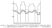
Turing 1952, Fig 3.
Our modern understanding of biological patterns started with a mathematical (and theoretical biology) paper by Alan Turing in 1952. In "The Chemical Basis of Morphogenesis", Turing's key observation is that a system of two components with specific interactions will form semi-periodic waves in space. An "activator" encourages the production of itself and an "inhibitor", which... inhibits the production of the activator. A critical aspect of this reaction is the relative diffusion rates of the components. The activator diffuses poorly, while the inhibitor diffuses readily. All of these characteristics can be described by a small set of differential equations.

Graphic edited from paper.
These differential equations indicate there will be no changes if the space being calculated over is entirely uniform, but the slightest irregularity results in dramatic changes. Regions with slightly too much activator grow and induce inhibition in neighboring regions. Regions with slightly too much inhibitor grow and induce activation in neighboring regions. Quickly the system stabilizes into a series of maxima and minima, visually forming spots/stripes of activation (or inhibition).
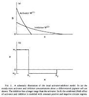
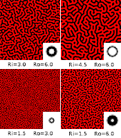
Young 1984, Fig 1.
Calculating the change of the activator and inhibitor concentrations over time become computationally expensive if we want to simulate a high-resolution system. Young described a simplification of the activation/inhibition system in his 1984 paper. Because the inhibitor diffuses more readily than the activator, we can think of the neighborhood around each active cell to contain two circular regions. The inner region is where the effect of the activator is dominant. The outer region is where the inhibitor is dominant. These regions can be simplified into two distinct circular regions with uniform activation and inhibition, respectively, instead of the continuous curves described by the differential equations. (Young 1984, Fig 1.)

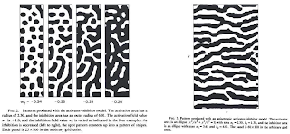
Young 1984, Fig 2 (left) & Fig 3 (right).
This simplified system is much easier to calculate over a large grid, as a cellular automata. For each pixel, any active cells in the inner region are activating neighbors, while those in the outer region are inhibiting neighbors. If a cell has more activating than inhibiting neighbors, the cell becomes active in the next turn. If a cell has more inhibiting than activating neighbors, the cell becomes inactive in the next turn. If a cell has an equal number of activating and inhibiting neighbors, the cell remains in its current state in the next turn. Depending on how you scale the active/inactive counts, you get a range of patterns. (Young 1984, Fig 2.) Applying the same simplification to an activator/inhibitor model with anisotropic (not the same in each direction) diffusion results in stripes. (Young 1984, Fig 3.)


I came across Young's model sometime while I was in high-school, roughly a decade after his paper was published. I was already playing with more conventional cellular automata using software I had written, so I added a module to play around with Young's model.
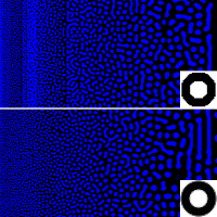
Fig d1.
One of the first images I produced (Fig d1) illustrates what happens when you bias the ratio of counted active/inactive neighbors. The x-axis biases the active neighbor count (from 0.0 to 1.0), going right. The y-axis biases the inactive neighbor count (from 0.0 to 1.0), going down.

Fig d2.
Next I tried scaling the neighborhood diameters. What I got was seemed to be a random association of diameters to pattern type produced. I didn't clue in to what might be going on until I calculated the effect of smoothly scaled diameters across a single image (Fig d2, top). I realized that the regions I had been using were aliased. Small increases in diameter were resulting in 'random' increases in the number of cells being counted in each region. After rewriting a bunch of code to use pre-defined neighborhood masks, I was able to confirm that using anti-aliased regions produced the pattern I had expected at the start (Fig d2, bottom).

Fig d3.
With the better way to define neighborhood regions, I started adjusting the radius of each region separately. I used some Fourier transforms of the resulting images to help me sort out what was going on, but I didn't save those figures. It turns out that the average feature size in the produced images is the same as the average of the two diameters used in defining the neighborhoods. If the two diameters are further apart, the resulting images show a greater range of feature sizes. By setting the region diameters appropriately, you can design the resulting image to have feature size and feature size variation characteristics of whatever you choose.
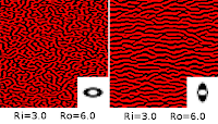
Fig d4.
It was also easy at this point to examine the results of anisotropic diffusion in the model. If both regions are squashed in the same direction, the resulting pattern looks more or less normal... only squashed (Fig d4, left). If the regions are squashed in different directions, stripes result (Fig d4, right.). I don't know what happens when anisotropic diffusion is applied to spots vs. stripes. I should explore that.
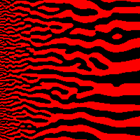
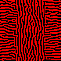
Fig d5.
Smoothly changing the size of the ellipse neighborhoods produces an appealing network of stripes of different thickness. (Fig d5.) This pattern reminds me of the pattern of stripes [sometimes] seen on the back of cuttlefish.

Fig d6.
Smoothly rotating the ellipses did not produce the results I expected. (Fig d5.) I played around with my code for a while, but never got diagonal stripes to form. I expect the problem is some artifact/bug in the code, rather than something intrinsic about the system, but I still don't know where. It might take rewriting the code from scratch to find my way around it.
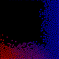
Fig d7.
Biological patterns are rarely ever so simple as the outputs of this model have been, so I attempted to simulate added complexity by calculating combinations of Young's model with different factors driving the interaction between one activator/inhibitor pair and another. (Fig d7.) In my example we see two different kinds of spots forming, with interesting interactions between them in the lower middle section.

One of the random interactions I simulated resulted in animated, mobile spots that would wander around the screen and occasionally replicate. Apparently, it doesn't take a very complicated system to start gaining some life-like features. Unfortunately, I hadn't written the program to display the random settings it had chosen. There was no way for me to save them. (I've since then rewritten the code to save any random settings. I will find those amoeba again!)


When I started graduate school, I had to set aside my explorations into theoretical biology like this. I'm now done with graduate school and find myself with sufficient free time to post to this blog, so I know I'll find the time to continue exploring the simulation of biological patterns.

Given the wide range of patterns seen in biology, I strongly suspect there are a great many more interesting results to be found exploring combinations of the simplified activator/inhibitor system described by Young's model.


References:

Tuesday, December 22, 2015

The Messy Science of Tardigrades

[Image source.]

Recently there has been some controversy in the news about the evolution of genomes in tardigrades. In particular, one recent paper claimed to see evidence for large-scale horizontal transfer of genes from bacteria/etc. into tardigrades, while another recent paper claimed to see no evidence for horizontal transfer.

The meat of the issue comes down to exactly how each group assembled the genomes they analyzed and published about.

Group 1:
  1. Illumina-seq (shotgun sequencing) with paired-ends.
  2. Notice lots of bacterial, etc. genes.
  3. Re-sequence genome using PacBio extremely-long-reads.
  4. Validate presence of bacterial/etc. sequences in tardigrade genome.
  5. Publish paper!
Group 2:
  1. Illumina-seq (shotgun sequencing) with paired-ends.
  2. Notice lots of bacterial/etc. sequences.
  3. Filter out bacterial/etc. sequences before constructing final genome.
  4. Publish counter-"paper"!

The first group first sequenced with paired-end reads using Illumina technology, then did re-sequencing using the extremely-long-reads of PacBio technology. This two-method sequencing allowed them to more reliably validate if the bacterial/etc. sequences were actually found contiguously in the DNA of the tardigrade or not. Any artifacts from one technique would likely not be found in the second independent technique. Any results shared between them thus have a higher confidence. The PacBio sequencing wasn't as comprehensive as the Illumina sequencing, so there wasn't complete validation of all cases of horizontal gene transfer. There is the potential that they've over-estimated the level of horizontal gene transfer. However, their methodology would allow them to see the difference between massive horiztonal gene transfer in the tardigrade's evolutionary history vs. the presence of contaminating DNA in the sample being sequenced.

The second group didn't put the same level of rigor into their sequencing. They used Illumina technology (as the first group), followed by intensive filtering of sequences which seemed to have an origin from contamination. They argue the bacterial/etc. genes seen in the first group's genome assembly were due to contamination. However, their result is exactly what would be expected from their methodology whether there was actually massive horizontal gene transfer in the tardigrade's history or not. I'm not convinced that their method would have been able to tell the difference.


A detail of the first group's results that lends credence to their interpretation over that of the second is that the bacterial/etc. genes found in the tardigrade's genome were not simply a random selection of genes as would be expected from a contamination origin. Instead, they were a selection of genes involved in DNA repair and stress response. These are exactly the sort of genes that would be expected to favor the survival of the tardigrades that had incorporated them.

Another section of the first group's results which were overlooked by the second was that the bacterial/etc. genes found in the tardigrades show evidence of having evolved inside the tardigrades for an extended period of time. The bacterial/etc. genes show a shift in the codon usage to be more like that of native tardigrade genes. As well, the bacterial/etc. genes have gained introns (something not found in bacteria). Both of these classes of changes would be very unexpected in a scenario where contamination was the source of the DNA.


The first group probably over-estimated the level of horizontal gene transfer in the tardigrade. The second group probably under-estimated the level of horizontal gene transfer in the tardigrade. So...  what is going on? This entire event shows very well how science is done in real life. Someone will have an interesting result. Someone else will produce an apparently contradictory result. Over time, the new results get closer and closer to telling us what the reality is.

The real world is messy. Science is, at its best, an attempt to understand what is happening in the world. It isn't telling people what should be, or what might be, but what actual is. The apparent uncertainty seen in regards to the tardigrades may confuse people who might be used to watching fictionalized representations of science that always seems to get everything right on the first try, or those who trust in science to get the right answer without realizing the extended process that getting the right answer can be. In the end, it is a good thing. All the interest the results in these papers has produced will likely inspire more research to be done which will add further clarity to what is going on in these interesting little creatures.


References:

Tuesday, December 15, 2015

Pain

You think you know pain. You've experienced pain all your life. You just might have probably broken a bone, or given birth, or been [mildly] electrocuted...  some of the more physically painful events that a person might think of experiencing.  If you're really unlucky, you may even now be living through the intractable, unending, pain that can be caused by cancer or some other disorders.

Some rare few people have no comprehension of your experience. They have a disorder called Congenital Insensitivity to Pain, or CIP. The disorder interferes with their ability to feel any pain. Not having to feel pain might sound like a nice idea, but pain is your body's way of telling you that something is wrong. Pain can get out of hand at times, but without it...  life gets difficult.

You learned a hot pan from the stove was not to be touched, because it hurt. You learned to take care while running, because it hurt when you fell. When you accidentally bite your tongue or cheek, it hurts and you [try to] avoid it again. Without pain, you would never learn any of those lessons. You would be severely burned, or break bones, or bite through your cheek and tongue. Pain is important, because it helps you learn to keep from damaging yourself as you go through life. People with CIP have very difficult childhoods, with their bodies experiencing damage at levels a typical person could never imagine.


Geneticists have studied families with high rates of CIP and have identified several mutations in the gene SCN9A. This gene encodes the voltage-gated sodium channel Nav1.7, critical for the normal transmission of signals along pain-responsive nerves. The same ion channel is responsible for the transmission of signals along olfactory nerves (Ahn et al 2011; ), so patients with the disorder also have an impaired sense of smell.

Researchers recently replicated one of these mutations in the laboratory mouse (Minnett et al, 2015). The resulting mice had no reaction to stimuli that should have caused a great deal of pain, without causing actual physical damage, like electro-stimulation. The mouse showed increased endogenous opiod activity. The introduction of the opiod antagonist Naloxone resulted in restoration of the mouse's ability to feel pain. A human subject with a similar mutation of SCN9A also showed a restoration of the ability to feel pain when treated with Naloxone, for the first time in their 39 years of life. The researchers are using their new knowledge to develop a treatment for intractable, chronic pain. The treatment would mimic the effects of the SCN9A mutation, by using a low dose of opiods paired with an Nav1.7 antagonist. This should allow for the effective management of pain with low doses of opiods, so avoiding the potentially-lethal side-effects associated with high-dose opiod pain-management therapy.

Not all cases of congenital insensitivity to pain are due to mutations in SCN9A. I found a paper (Manfredi et al, 1981) which describes a patient who had no pain response, but did not have an impaired sense of smell. This ability to smell indicates the patient had a functional SCN9A gene. The patient was also described as not showing a restoration of pain sensation upon treatment with Naloxone. My reading of the 2015 paper suggests the authors didn't realize that Naloxone would restore pain sensation in their patient. It looks like they missed this critical knowledge that was known in the 1981 paper when they were doing their literature research for the project. The 1981 patient may have a mutated NTRK1 gene, another known cause of congenital insensitivity. The state of research in 1981 didn't involve the intensive genome sequencing needed to identify mutant genes, so it remains unclear.


Did you catch the problem in this story?

The 2015 paper indicated the patient had never experienced pain until the researchers realized that Naloxone might be a treatment for their disorder. The 1981 paper described an interesting patient with congenital insensitivity to pain who, surprisingly, didn't respond to Naloxone. Naloxone has been known as the treatment for this disorder for more than thirty years.

The patient described in the 2015 study has lived through 39 years without a medical professional giving them the known treatment for the disorder that resulted in them experiencing the extreme physical damage that the disorder leads to. The treatment could have normalized their pain responses and prevented the damage. Because of the diversity of underlying biological causes to different cases of CIP, Naloxone treatment may not work, but it is readily tested and has minimal side-effects.

This disorder impacts maybe 100 people on the planet. It receives very little research attention, even though it is a relatively charismatic disorder, so it is understandable that critical knowledge might occasionally be forgotten or not communicated to those who should know it. That the re-found knowledge of the 2015 paper is being used to develop a treatment for the intractable pain experienced by many people across the world is a wonderful thing. It really could improve the lives of millions of people by removing their chronic pain without needing powerful and dangerous drugs. However, It still makes me very angry that the patient in the 2015 paper wasn't given appropriate treatment for most of their life with the disorder.


References:

Tuesday, December 8, 2015

More Convergence on the Seaside

Cakile maritima on a southern California beach.
(I know this one is tasty, in real life.)
In a previous post (the-biologist-is-in.blogspot.com/2015/03/convergence-on-seaside.html), I discussed two seaside plant species that both have succulent, edible (and reportedly tasty) leaves.
Cakile maritima (Sea Rocket). [Brassicaceae, annual]
Crambe maritima (Sea Kale). [Brassicaceae, perennial]
Since then I've found a selection of other seaside plant species that all have succulent, edible leaves.
Blutaparon vermiculare (Silverhead, Saltweed). [Amaranthaceae, perennial]
Cakile edentula (Sea Rocket). [Brassicaceae, annual]
Cakile lanceolata (Sea Rocket). [Brassicaceae, annual]
Crithmum maritimum (Sea Fennel, Rock Samphire). [Apiaceae, perennial]
Eryngium maritimum (Sea Holly). [Apiaceae, perennial]
Limbarda/Inula crithmoides (Golden Samphire). [Compositae, perennial]
Salicornia bigelovii (Marsh Samphire, Dwarf Glasswort). [Amaranthaceae, perennial]
Salicornia europaea (Marsh Samphire, Glasswort). [Amaranthaceae, perennial]
Salicornia virginica (American Glasswort, Pickleweed). [Amaranthaceae, perennial]
Salsola soda (Barba di Frate, Agretti, Liscari Sativa). [Amaranthaceae, annual]
Sarcocornia quinqueflora (Beaded Samphire, Beaded Glasswort). [Amaranthaceae, perennial]
Sesuvium maritimum (Annual Sea Purslane). [Aizoaceae, annual]
Sesuvium portulacastrum (Sea Purslane). [Aizoaceae, perennial]
Tecticornia arbuscula (Shrubby Glasswort). [Amaranthaceae, perennial]
Tecticornia pergranulata (Blackseed Glasswort, Blackseed Samphire). [Amaranthaceae, perennial]
What is it about the seaside environment which is selecting plants to be succulent and edible? I've got some thoughts that I think lead to a partial answer. Let's break down the question into two parts.

Why are they succulent? The seaside substrates where these plants grow is typically composed of sand, gravel, or rock. These substrates don't hold water at all. Even though there is an ocean very nearby, any small plant growing above the high-tide line is effectively growing in the middle of a desert. Two main strategies for this situation are 1) grow extremely deep roots and 2) hold onto any water that they find. The first strategy is typified by Creosote (Larrea tridentata) and Mesquite (Prosopis spp.), neither of which would be described as edible. The second strategy of holding onto their water, means a plant will be succulent in some way or other. There are plenty of both toxic and edible succulent plants, so there is more to the story.

Why are they edible? Some of the plants are perennial, while others are annual. Before I started looking into it, I was thinking they were all weedy species. Weedy plants (or animals) are those that invest a lot of their energy in reproduction, while investing very little in self-defence of any specific individual (r-selected). For plants, this means they're typically annuals (or short-lived perennials) that don't invest much biological energy into growing spines, fibers, or poisons. In short, r-selected plants are more likely to be edible to generalist herbivores like ourselves. Now, that none of these species would count as a long-lived perennial (like a woody shrub or tree) may perhaps mean that the weediness argument has some value in understanding this group of plants.

Before I started looking up these species, I had never heard the name "Samphire" before. The name seems to be used generally for any succulent (and edible) weed growing on a rocky seaside of the northern British Isles. Several of them are described as being easy to grow in a garden setting. Some of the plants can grow directly in sea-water. These may be a bit trickier to grow in the home garden. I like growing interesting plants, so hopefully I'll be able to try growing some of them over the next several years.


References:

Tuesday, December 1, 2015

Evolutionary Battle of the Sexes

Most of the familiar animals are found in male and female versions. Some others switch between male and female and then there some are both at the same time. Plants mix it up a bit. Most of the familiar ones are both male and female at the same time, with gender-specific sex organs packed together into flowers. Some others have separate male and female flowers. Still others follow our pattern, with separate individuals being male and female.

When the two genders are split into different organisms, an interesting evolutionary dynamic comes into play:
  1. Suppose male births are less common than female.
  2. A newborn male then has better mating prospects than a newborn female, and therefore can expect to have more offspring.
  3. Therefore parents genetically disposed to produce males tend to have more than average numbers of grandchildren born to them.
  4. Therefore the genes for male-producing tendencies spread, and male births become more common.
  5. As the 1:1 sex ratio is approached, the advantage associated with producing males dies away.
  6. The same reasoning holds if females are substituted for males throughout. Therefore 1:1 is the equilibrium ratio.
This simple chain of logic is often attributed to R. Fisher (as "Fisher's Principle"), but originates in an older paper by W. D. Hamilton. The consequence of this is that we would expect species to have the 1:1 equilibrium ratio. Any species that doesn't fit this pattern... become interesting. They don't follow the pattern because something else is going on.


A Dandelion on an Alaskan peak.
Dandelions (Taraxacum officinalis) are interesting. Bees collect the male pollen and distribute it to the female pistils, as with most flowers, but the Dandelion diverges from the common pattern at this point. The pollen induces seed development in a process called apomixis, where the resulting seeds show no genetic contribution from the pollen. Each Dandelion is a clone of its female parent, so the population is at an extreme 0:1 male to female ratio. Any genetic elements that would increase the chance of male genetics contributing to the next generation would have a severe evolutionary advantage, but the males have completely lost the fight.

The Dandelion female 'parent' invests far more energy in producing seeds than the male 'parent', so writing the male entirely out of the genetic equation may not be so strange in the end.

Saharan Cypress (Cupressus dupreziana) represents another extreme case... but in the exact opposite direction. The seeds of the Saharan Cypress show no genetic contribution from the mother. The plant will even act as a surrogate for pollen from the related Mediterranean Cypress (C. sempervirens), producing baby C. sempervirens plants. That C. sempervirens will also play the surrogate role for C. dupreziana pollen, producing baby C. dupreziana plants, says that the behavior is probably seen more generally in this group.

Writing the female entirely out of the genetic equation is a very strange concept. Given that it is the female parent that invests so much energy into seed production, the female genetics should remain important.


If you've followed along so far, you might not have noticed I pulled a fast one on you. Hamilton's logic works in mammals like us because we have distinct genetic elements that are associated with the male and female genders. Genes on the Y-chromosome or on the X-chromosomes can selectively respectively favor the male or female gender. Most plants produce both male and female gametes and so there are no genetic elements that are associated with either one in particular. This disconnect is probably what has allowed plants with such extreme reproductive patterns to have evolved. Because no genetic elements would be stuck with only one gender parent, there is no selective force to maintain parity of genetic transmission through both genders. Genetic influence passing through female gametes or male gametes alone then becomes as viable as any other mechanism of vegetative reproduction a plant may use.

Though Dandelions are the traditional example of apomixis, not all Dandelions use this strategy. There are versions that have a more typical sexual pattern (and the difference seems to come down to chromosome copy number). The Cypress also sometimes mixes up the genetics from pollen with those from eggs. Thus both types of plants persist in generating some of the genetic diversity needed to survive in the long-term race against the Red Queen (the-biologist-is-in.blogspot.com/2014/04/oxalis-and-red-queen.html), even if they go about doing in a peculiar way.


References: